Perceptron
A perceptron model trained to classify sentences as positive or negative. Three optimization methods are compared: Gradient Descent (GD), Stochastic Gradient Descent (SGD), and Adam. Another goal is to learn how a perceptron, building block of neural networks, work by building it from scratch. Dataset consists of 400 sentences, 20% used for testing and the other 80% for training. Most of the dataset generated by using LLMs. 200 positive and 200 negative sentences. You can see some example sentences below:
[neg] The echo of a closing door resonated with the finality of an ended chapter.
[neg] The hollow echo of footsteps in an empty hallway underscored the solitude.
[neg] The once-lively room now felt like a cavern of echoes, devoid of life.

[pos] The shared excitement of a surprise event brought smiles and expressions of awe.
[pos] A successful surprise party left the celebrant beaming with happiness and gratitude.
[pos] The sound of rain tapping on the roof created a cozy atmosphere for an evening indoors.
The core logic of this project is built in C from scratch. Python is only used for preprocessing data and generating images. Check the source code for more information. You can see a portion of the report I wrote for this project below.
Pipeline
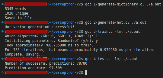
Compile and run the numbered C files in order, following the on-screen instructions:
- generate-dictionary.c
- generate-hot.c
- train.c
- test.c
Model
The model is defined as:
y = tanh(WX)
where W is the parameter vector and X is the one-hot vector of a sample. The output is rounded to -1 or +1 to produce a binary prediction.
Training supports three optimization methods: GD, SGD, and Adam. Charts are generated using Python and matplotlib. Methods are capped at 1000 iterations with a step size (EPS) of 0.1.
Training Results
Comparisons were made across five different initial parameter values. Below are selected results.
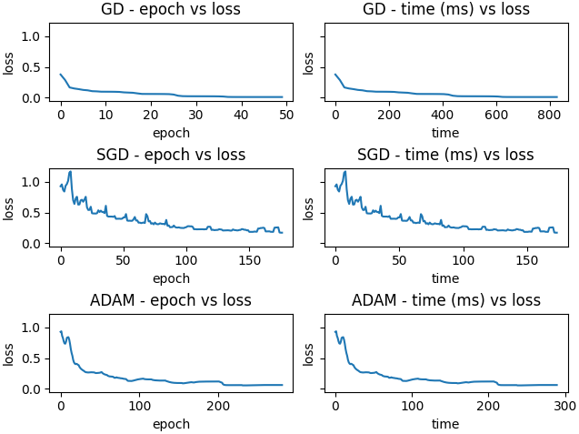
Random initialization
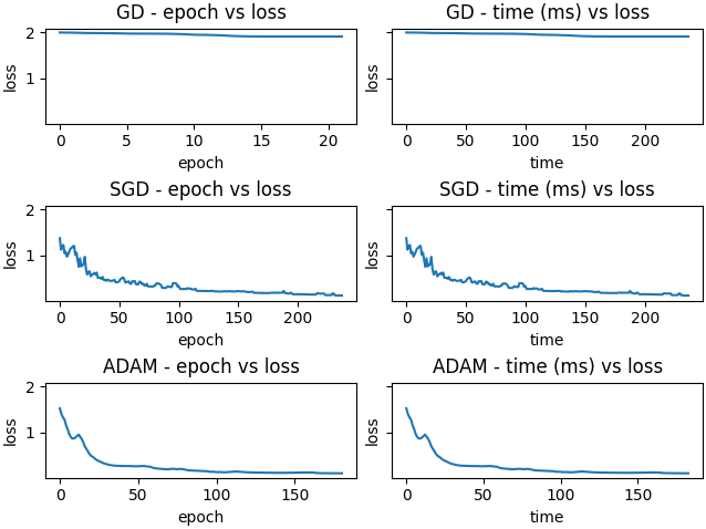
Adam is the most efficient method in both iteration count and runtime. GD gets stuck in a local minimum, while SGD escapes it by randomly selecting samples and Adam escapes via momentum.
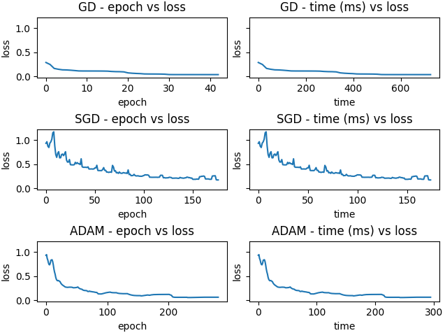
Initial parameters: 0.001
Initial parameters: 0.1
GD gets stuck in a local minimum again.
Initial parameters: 0.5
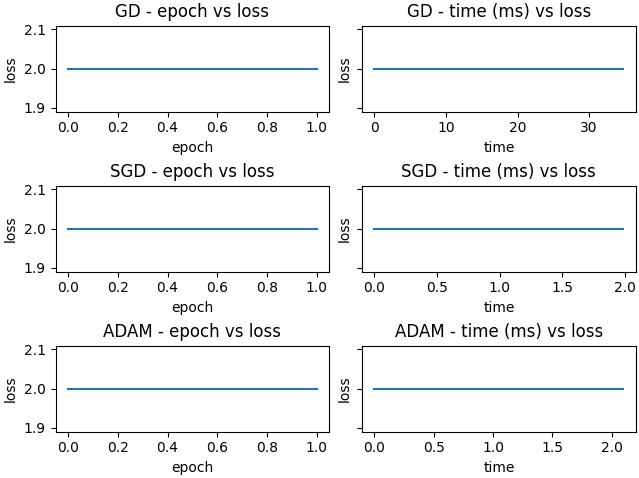
Gradients vanish due to the high initial values, so no updates occur and all methods converge on the first step.
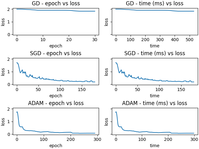
Initial parameters: 0
Adam is again the most efficient. In this case, each GD iteration takes roughly 16x longer than Adam.
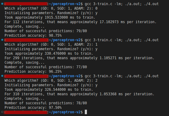
Testing
The model is evaluated on the held-out 20% test set. Settings: 1000 iteration limit, EPS = 0.05, random initialization.
2D Visualization of Optimization
Since the parameter vector has 1000+ dimensions, it cannot be plotted directly. PCA first reduces it to 50 dimensions, then t-SNE reduces it to 2. The plot below shows SGD training from 5 different starting points (1500 iterations, EPS = 0.01), generated with plotly, scikit-learn, and numpy.
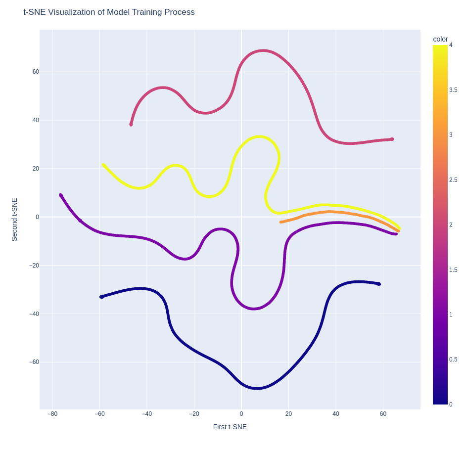
| ID | Initial value | Color |
|---|---|---|
| 0 | 0.01 | navy |
| 1 | 0.001 | purple |
| 2 | -0.03 | pink |
| 3 | 0 | orange |
| 4 | -0.0009 | yellow |
Runs 1, 3, and 4 converge to the same local minimum. Runs 0 and 2 converge to different local minima.
Conclusion
Among the three methods tested, Adam consistently outperforms GD and SGD in both iteration count and wall-clock time. GD is prone to getting stuck in local minima regardless of initialization, while SGD and Adam are more robust. At high initial values (0.5), all methods fail to make meaningful updates due to vanishing gradients, which highlights the importance of careful initialization.
The t-SNE visualization confirms that different starting points can lead to different local minima, and that convergence behavior varies significantly across runs even with the same optimizer.
Overall, building the core in C kept the implementation lean and fast, and the Python tooling made it straightforward to analyze and visualize results.